If you’ve been working with Data Science I’m sure that at some point you needed to try a lot of different things to solve a problem. At the same time, you also needed to keep track of the performance of what you tried to do.
Projects, experiments & Spreadsheets
Probably at some point you, like me, fired up an Excel spreadsheet and tried to manually keep track of things. This often results in chaotic organization both in the project folder as well as the spreadsheet itself.
It is hard to keep track of all possible things that can run differently in an experiement. Preprocessing steps for specific models, the models themselves, the parameters,…
MLflow comes in to help sort this kind of thing. It is a platform built to organize, facilitate experimentation, streamline and serve models to production. Basically a platform to manage ML lifecycle.
Quick stop before we move forward, you can read this on Medium as well
A (Brief) Intro to ML Flow
As of this writing, MLflow has 5 components in total. For this quick guide I’ll use only a few of the available ones (highlighted below), which are:
- Tracking
- Models
- Model Registry
- Projects
- Recipes
The Tracking module acts pretty much as a logger, but for everything model related: What model is being used, which parameters are configured in the run, outputs (even tabular and images), etc.
Tracking has many “flavors” — how common ML/AI libraries such as sklearn, Keras, H2O are named — to help store important data and metadata of commonly used libs.
Models is a form of wrapping a model after training. It encapsulates a model in such a way the model can be saved, containerized or accessed easily to be ran in other environments or easily called.
Model Registry is the logical next step of the Models wrapper. It enables to register models that are useful and will be used in production. By registering the models, we can perform version management to them. This makes it easier to organize and register the production pipeline of a model.
MLflow tracks, throughout the components, basically 3 things:
- Models: model objects that can be agnostic or belong to a certain flavor of ML/AI library;
- Parameters: Constant values related to the models (e.g. the weights of a Neural Network);
- Artifacts: Every sort of file generated in a run. You can, for instance, save an image (like the plot of a DecisionTree) or a table.
These objects are tracked in a run level within an experiment. An experiment is a general environment for MLflow to store information. A run happens within an environment. A run is pretty much the name MLflow gives to an algorithm execution.
To centralize all components and facilitate usage, MLflow has a really intuitive UI that can be easily started from the terminal.
MLflow can store all its files and artifacts locally. But, you can use a DB such as PostgreSQL to log the artifacts. For my tests I left it saving the data locally. In this case, MLflow generates a mlruns folder in the directory of the project that I supress in the repo using .gitignore.
A Quick Problem for a Quick Start
To try out MLflow in practice I used a basic dataset to solve a straightfoward problem. I’ve used data sourced from Amazon made available in Kaggle to predict the sales amount for certain groceries in the UK. You can find the data here.
The main focus of this test is to understand and use MLflow. So, for this purpose, only basic data cleaning was performed. Let’s get into it.
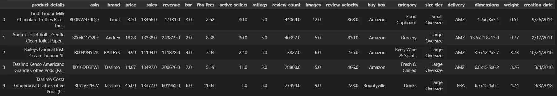
First things first, let’s get a sense of the data at hand. We have data for over 6.000 products that contain some features regarding the product itself as well as its performance in the marketplace (e.g. price, sales, revenue, …). See an example below:
We fetch the raw data and after some cleaning, feature engineering and subsetting we end up with a little over 5.000 products with the following features:
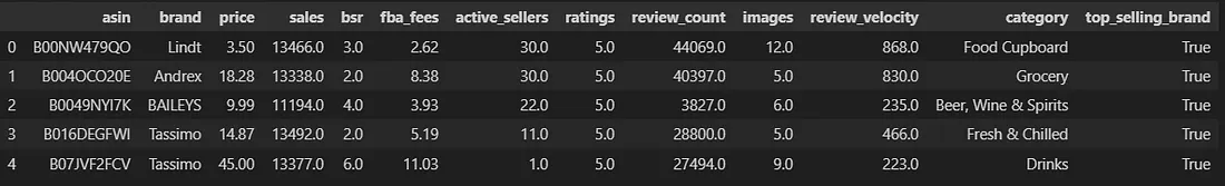
With this data, we can start running models for the sales column. Keep in mind not all the features in the picture above will be used. I’ll be using a simple Linear Regression as a baseline for comparison with other models (and to help show the power of MLflow down the road).
Using MLflow
MLflow can be installed as a library in your pip or conda environment. So you can bring up a terminal and run:
pip install mlflow

# or, if using Anaconda/Miniconda:

conda install -c conda-forge
I’ll be using sklearn. I can simply import mlflow to use it in my code. With it imported I can use the following logic to track my models:
# Other imports #
import mlflow

mlflow.autolog()

### Data ingestion ###
### Sklearn stuff ###

# Baseline Model
with mlflow.start_run() as run:

    lr.fit(X_train, y_train)

    y_pred = lr.predict(X_test)

    mse = -1 * mean_squared_error(y_test, y_pred, squared = False)
    mae = -1 * mean_absolute_error(y_test, y_pred)
    r2 = r2_score(y_test, y_pred)

    print('Logging Baseline Linear Regression Results')
    mlflow.log_metrics({'Neg. RMSE':mse,
                        'Neg. MAE':mae,
                        'R2':r2})
Note: keep in mind that MLflow has .autolog() methods for common flavors, but they work best up to certain versions. Check if your lib version is fully supported by autolog, if you’re going to use it. It won’t break your code necessairly, but it can lead to problems.
I associate the code to my experiment with my mlflow.autolog() call. It automatically identifies I’m using sklearn (but I could use mlflow.sklearn.autolog()).
Then, I use a context to call mlflow.start_run() to start a run in the experiment. The run in the snippet above is for the baseline LinearRegression().
If you opt to start a run outside of a context, just make sure you end the run explicitly after.
By calling .fit(), MLflow automatically identifies the command and logs training metrics. I will also manually log using mlflow.log_metrics(). Within that run the Negative RMSE, Negative MAE and R2 scores are logged. This is done to enable comparison with test performance with other models.
The reason to use Negative RMSE and MAE and not their positive (and most usual) counterparts is that I want to perform Hyperparameter Tuning with GridSearchCV. To work within the search, these metrics need to be negative.
For the GridSearch, we use the same block used for the Linear Regression. The only change is to call the Cross Validation object instead of the model when we run .fit() and .predict(). MLflow will automatically handle what happens on the backend and will log the runs apropriately for the CV case.
Tracker
Now, let’s see how this looks after running in the mlflow UI. To start it just bring up a terminal window in the environment you have it installed and type:
mlflow ui
This will prompt you with a local IP adress where the UI was served to. You can open it in your browser to find the following page:
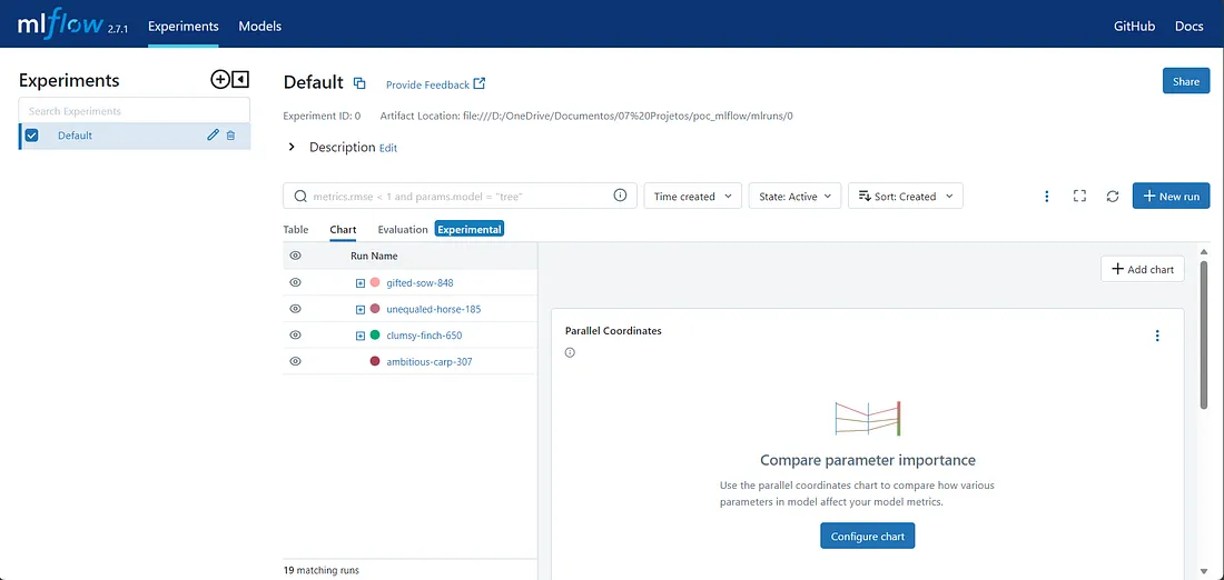 Initial screen of MLflow
After running the models this is what we have. On the left, we have a list with all experiments. In this case we only have one called “Default” (automatic name assigned by MLflow, you can change it).
Using mlflow with autolog out of the gate will associate the runs to this experiment. You can build different experiments in the ui or through the API within the code.
On the right, we have a list of all of our runs. Each run gets one of the assigned names. One for the baseline model (ambitious-carp), one for the 3 other models I’ve used, these with Hyperparameter Tuning.
Notice how the GridSearchCV objects will have a “+” to their left. If we expand, we will have the 5 best performing combinations in the GridSearch! The top-level run, that encapsulates all the other runs, will be the best estimator. This would be equivalent to a .best_estimator_ call within sklearn.
Now with the models tracked, using the chart tab, we can can visually answer 2 questions:
- Do the models outperform the baseline?
- Which model performed the best?
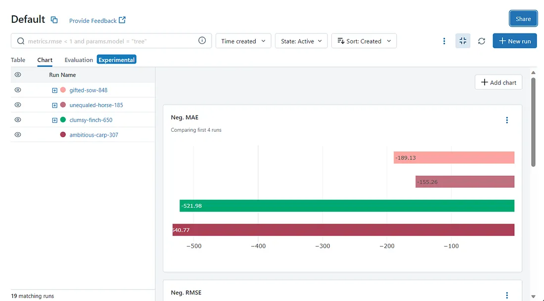 Example of Metric Graph by Run in MLflow
Using the Negative MAE as example, we can see one of the strenghts of MLflow. All of our models, even the ones with tuned hyperparameters, can be easily compared side by side for any of the metrics we logged.
This view enables us to answer both questions above. We do actually outperform de baseline (last deep-red bar), and we see that the second model (name: unequaled-horse) is the one that performs the best. This is true for all 3 metrics we’ve tracked.
Let’s then take a deeper look into the best model by simply clicking on its name on the list. We will this way access the second component.
Model
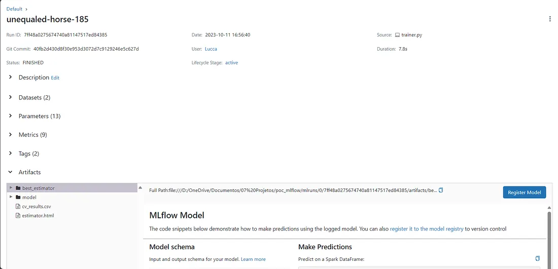 Detail of a run
This is the page that describes a run, that contains a model object. Notice how it has a lot of attributes: The data used to train and evaluate it, the parameters, the metrics tracked and the artifacts.
The “artifacts” section is what actually holds the model container. MLflow shows us how is the schema for the data used in the model and how we call the model to make predictions, with code snippets. We will do that just in a bit.
First, I will register the model to see how the Model Registry works. We can register a model by simply clicking on the “Register Model” button and giving it a name. After it’s registered, we can access the “Models” tab in the UI.
Registry
 Details of a registered model
The initial screen of the registry will be a list of the registered models and their names. By clicking on a model, the screen above pops up.
Notice how a model will have versions. The first version we generate is, naturally, Version 1. To generate a second version of a model, just log a model with the same name it has in the registry.
We can also add a description and information about who generated it. But what is really interesting here, along with the versioning possibilities, is the “Stage” tag.
With it, we can assign if a model is in Staging or Production phase. To change it, we simply click on the version we want to edit and select the correspondent stage. Notice how we also have the schema, source run info and also tags we can associate to our model. I’ll put my model on “Staging”.
It’s also worth to notice that changing the stage will trigger some actions in MLflow. For instance, when we transition a model to “Staging” a prompt shows up asking if you want that other models that get to “Staging” go to “Archived”.
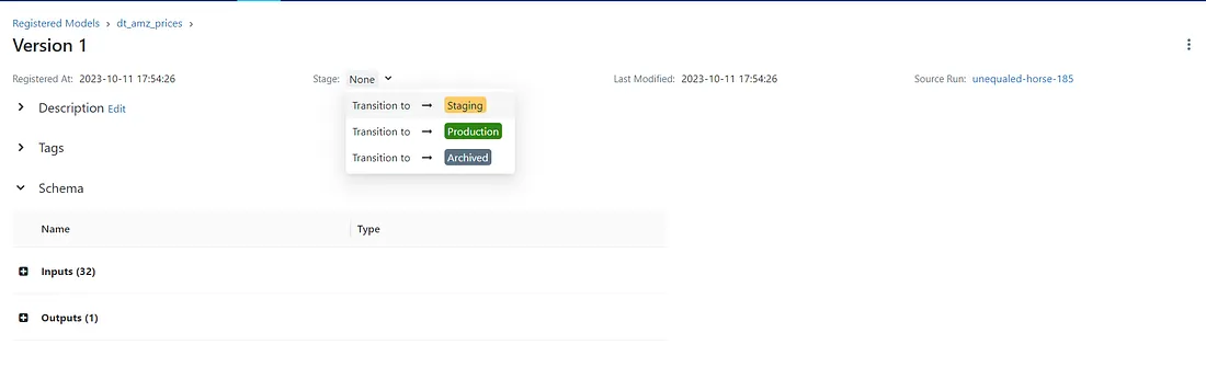
Trasitioning registered model version to Staging With our model registered, we can call it easily to predict on data.
Calling a Model
To call a model you need to basically pass a URI string to mlflow. There are many options to do so, I chose one that seemed the most clean and intuitive to me. Feel free to check out other options on the docs.
To call my model to predict on data, I can simply do:
model = mlflow.sklearn.load_model('models:/dt_amz_prices/staging')

# Given that the data corresponds to the Schema in the model
y_pred = model.predict(X)
And the trained model will run. That’s it. MLflow enables us to easily compare, share, store and use a lot different models for any given ML problem.
This has been, of course, a simplified scenario that I used to grasp how its basic functions work. We could, very easily, also serve this registered model as an API. However, this is beyond the scope of this text.
Final Thoughts
This text is a product of my personal studies to understand MLflow. I’ve used it to solve a quite simple ML problem. This was done as a way to understand how its functionalities help Data Scientists experiment in a more orderly and structured fashion.
I’ve covered 3 of the 5 components of the tool and tried out how they can be used in a project setting. In my honest opinion, MLflow is something I am strongly considering to adopt as a standard for my own work. This is because of the following reasons:
- Structure: I can test various models, with various configurations really easily, in a ordered way that I know where what is;
- Easy comparability between runs: I don’t have to build extra layers of code to keep track and compare all the experiments I run. The chart mode helps a lot for model selection and comparison;
- Replicability: It’s easy to call any model, not only the registered, without the fuss of opening other files and replicating the code (given the data preprocessing is the same);
- Transparency : At all times we can look at parameters, features, inputs, outputs and artefacts from every model. If in a team setting you can see who did what;
- UI: The UI is a major facilitator. It is clean, simple and self explanatory. This helps a lot to navigate problems with many possible solutions. I hope this text helped you understand the main strenghts I’ve come to experience using MLflow.
Acknowledgements and links
- For the full code of the project, check out my Repo on GitHub.
- Check out the MLflow docs for further and more in-depth information.
- The data for the project came from this dataset on Kaggle. If you liked the text, leave some claps, a comment and feel free to check out my personal page here