I consider myself somewhat of a regular traveler. That’s why I often look for places to stay in AirBnb. But, when I fire it up, the options are countless. Don’t get me wrong, the filters on the site are great and I always liked it. But as a Data Scientist, I wonder if even with some simple Data Analysis navigating AirBnB could be made easier.
That’s why I asked myself if I could use Rio de Janeiro’s (my hometown and a popular tourist city) AirBnB data to:
- Find out if I could narrow my search by looking directly into the cheapest zones and cheapest neighbourhoods into each zone.
- Discover natural listing groups (i.e., clusters) based on their declared characteristics so that, if I wanted to, I could look into the group that suited me the most for a trip.
- Find out which are the most (and least) common ammenities I should expect when looking into listings in Rio.
Let’s get into it.
Quick stop before we move forward, you can read this on Medium as well
Sometimes I don’t want to spend that much
Price is an easy go-to filter. But that isn’t the only factor to take into consideration in a travel. You might wonder about distance to touristical spots, public transportation or even if you are cutting a good deal for that region… Location matters.
So to get a glimpse of that, we can try check out the prices by neighbourhood and even by city zone and see if they vary and, if so, we can rank them from cheapest to most expensive.
The data I had at hand didn’t contain city zone information. But we won’t let that stop us. With an easy scrape using Pandas read_html method on this Wikipedia page, we can get the city zone data to populate our table.
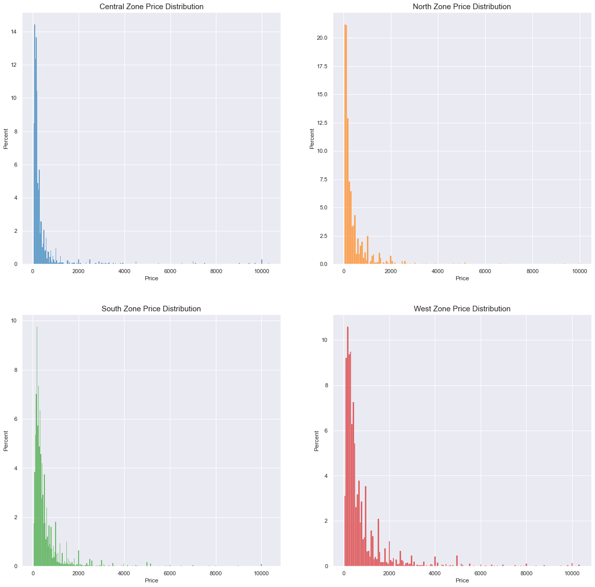
So first let’s take a look into the price distribution for each city zone:
 This is a caption
Note: y-axes are not shared between plots
We can see that generally price is a right-skewed distribution and that zones have effective differences in their distribution behaviour. For instance the south zone peaks more to the left then the north zone. West zone has a fatter tail.
This gives us two informations: We can group regions and use a comparison metric since it most probably will wield different results. Given the distribution, the median will be used. This results in:
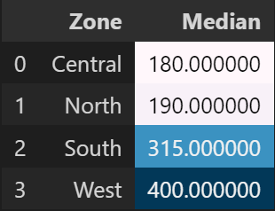
So when looking for a place to stay, listings on the North and Central regions might be more price-friendly.
We can dig a little bit deeper and even, for each zone, list the neighbourhoods within each region that have the cheapest prices:
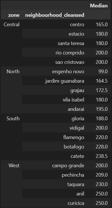
This is where some domain knowledge kicks in, though. Especially on the West Zone, the cheapest lisitings are really far away from the downtown or touristical spots.
But we have considerable price differences even within the cheapest/ expensive regions. So bringing this geographical layer on top of prices (and vice-versa) might facilitate users navigating through listings.
But what if I’m looking for something in specific?
Maybe location doesn’t matter as much if your priority is to first find listings suitable to your needs. That’s where clustering comes in. We can find natural groups of listings with similar features for someone can look into without the need to filter variable by variable.
The variables that describe a listing can be interpreted essentially as categorical. It can be argued that something like the amount of bathrooms a listing has is continuous/numerical, but on the sample it was rare to have more than 3 bathrooms in an AirBnb listing, for example.
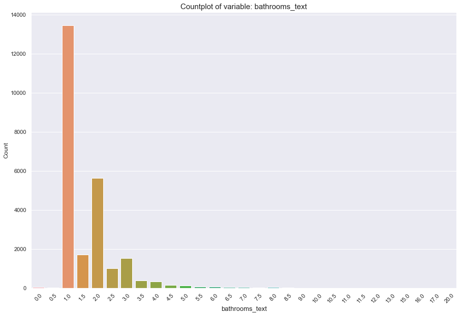 Count of listings for the bathroom variable. Note that from 3 bathrooms onward, there are few listings that contain more baths. There are even listings with no bathrooms!
What we see for bathrooms happens generally for the other variables that describe listings as well.
This limits our approach to categorical variable clustering methods. For this one, I will be using KModes. But you could use some variation like Gower Distance + Hierarchical Clustering.
After selecting our desired variables: Room Type, Number of Persons Accomodated, Bathrooms, Bedrooms and minimum accepted nights we can use our methods’ cost-function to set up an elbow-method plot and define our n for our clusters.
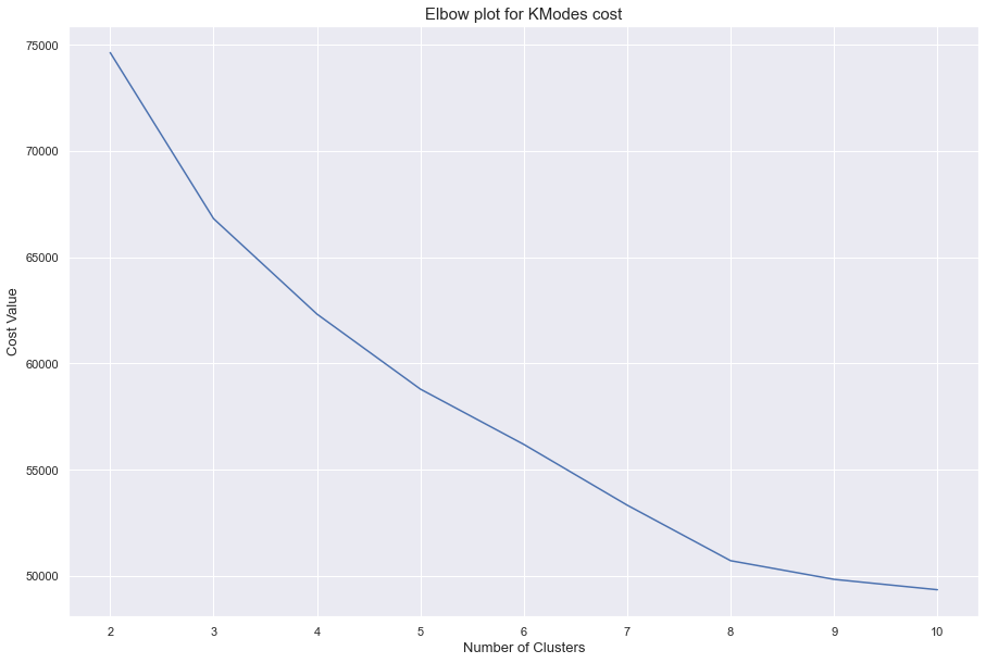
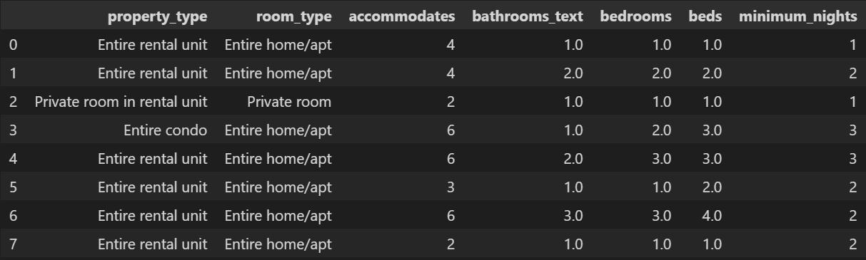
It looks like n = 8 is a nice enough amount of clusters. The rate in which the cost falls after that slows down heavily. When we run it we get the following clusters (using their centroid as reference):
 Clusters
Centroids, in this case, are the most-frequent value for each feature.
It is normal that most clusters are centered around Entire rooms/ apts in Entire Rental Units. These values dominate the dataset, having more than 50% of listing associated to them.
The biggest differences come from the “size” of the listings and the minimum nights. With size I want to express how many people they accommodate and the amount of bathrooms, bedrooms, etc. that a listing has.
If users were to search for listings in a city, the clusters could be a good starting point for showing them listings more aligned with their needs.
What if I want WiFi in my room?
Sometimes you want certain amenities. Sometimes you expect a room to have some basic things. So, it is only natural to try to find out what are the most common and rare amenities in listings. That way, users could know what to expect (or not to) for the listings in the city.
To start off answering our final question, we look into the the amenities field available in the dataset. It is a somewhat tricky feature. It is a whole string that should’ve been a list. So it is a list contained within a string and a simple .split() won’t cut it.
With a little bit of RegEx and text cleaning, we get our data to a list format. The only thing left to do is some text cleaning especially for WiFi. Since it’s is an important aspect nowadays, we do some special cleaning for it. WiFi values have multiple values like:
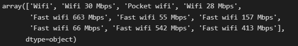
Multiple different forms to write that a listing has WiFi
With the cleaning handled, we can use the .explode() method to turn our lists into rows and make our analysis easier.
We get a total of 2788 unique amenities. But, considering each amenity is only listed once per listing, we can use .value_counts() on top of our exploded dataset to get the number of listings each amenity was cited in. This allows us to approach the problem using a Pareto logic. That is, a low number of amenities will show up with high frequency.
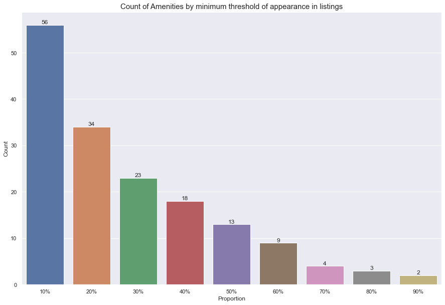
We can see that even by making a cut as small as 10% on the proportion of listings an amenity shows up in, we already reduce the amount of amenities from 2788 to 56.
I chose to work with this this 56 amenities subset. Considering that there might be a lot of amenities that will show up sparsely or are super specific, we cannot simply select the overall least cited amenities. This could lead to unnecessary/ wrong information.
For instance, it is safe to assume that a refrigerator from a specific brand (which exists on the data) is not an amenity someone would actively look for. Even the least common amenities must be contained in a group within reason.
With that in mind we get that:
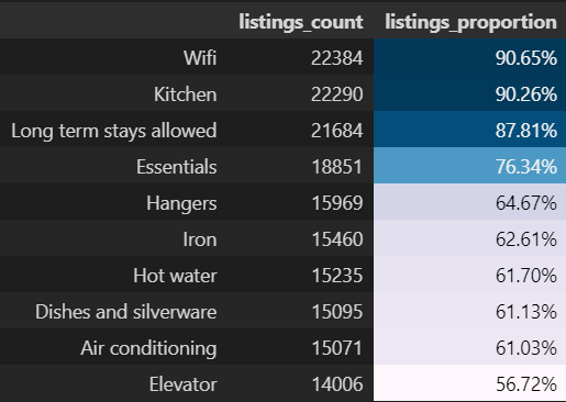
Are the most common amenities, so you can expect them to occur in a lot of the listings. Need WiFi? You’ll probably have it covered. No need to worry about it.
On the other hand:
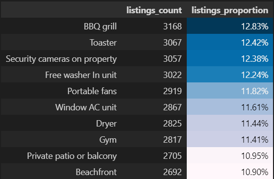
Are the least common amenities within that subset. So if for instance a beachfront view is a must for you when coming to Rio, you might only have more niched options available.
Conclusions
All things considered, all 3 analyses show relatively simple ways data could be incorporated to facilitate decision-making within the platform for the users. If we get back to our starting questions:
- We can narrow our search for cheap listings by adding a geographical layer to our data. This could be even further explored if we incorporated more data like proximity to tourist sights or restaurants concentration , for instance.
- It is possible to segregate listings based on their declared characteristics like amount of beds, rooms, etc. using a relatively simple clustering algorithm. This might be helpful to present to users more focused listing groups in-line with their needs without the need to manually set filters.
- From more than 2000 amenities we can get a subset of 56 significant amenities that could allow a user to catch a glimpse of what they could expect in a lot of the listings or not. That way, expectations can easily be set.
Naturally, all three paths could be enhanced with more work put into them. But the conclusions show how already on the current state we can create value to an user by answering key-questions and focusing of efficient analysis methods.
Acknowledgements
The full notebook and data can be found on my GitHub.
Data for AirBnB was collected from Inside AirBnb.
For more references into K-Modes, I recommend visiting nicodv’s GitHub that contains not only the implementation of the algorithm but references to the Theory behind it.
This work was done as a submission to Udacity’s Data Science Nanodegree Program.